Activation Functions for Neural Networks

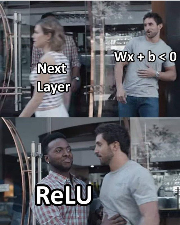
Image source

I’ve recently started volunteering with DataKind SF, and will be working on a computer vision project for an organization that wants to use satellite imagery to locate poor households in need of water subsidies. Since I haven’t worked with image data before, I wanted to take a few weeks to prepare by improving my deep learning skills, and learning more about visual feature extraction and image classification. So, I’ve been working through the deeplearning.ai Deep Learning Specialization on Coursera.

This blog will cover activation functions for neural networks, and is the first of a series covering the relevant information from the specialization that I want to make sure to remember, supplemented with additional learning from outside the course.

Neural Network Structure

Fundamentally, neural networks are composed of a series of interconnected “neurons” (individual processing units), which are organized into layers. The input layer receives the data, and the output layer determines the predicted values.

In between exist one or more “hidden” layers, which is where most of the computation takes place. The neurons in each layer are connected to the neurons in the next through channels, each of which is assigned a numeric weight. The neurons of each layer also have a numerical value, called the bias.

At each layer the input values are multiplied by the weight, and the bias is added. This new total is passed through an “activation function” before the data is set to the neurons of the next layer. Typically this activation function is the same for all hidden layers in a neural network, and has a large impact on the model’s performance and efficiency. The addition of an activation function is critical for helping the neural network to learn non-linearities in the system, since otherwise neural networks are essentially just linear models, and may not be able to model more complex relationships.

This process of the data being fed through the network is called forward propagation. At the end of one pass of forward propagation, the output layer determines the prediction. The output layer also has an activation function – which is typically different from the one used in the hidden layers – that is dependent upon the type of prediction required by the model.

During training, the model compares the real target value to the predicted values according to some loss function, and adjusts the weights to improve the prediction through back propagation (covered in detail in my calculus blog), in an iterative process.

Activation Functions for Hidden Layers

There are many possible choices of activation functions for hidden layers. Some of the most common include Sigmoid, hyperbolic tangent (Tanh), and ReLU.

Note: The activation function plots in this blog are all taken from this page

Sigmoid

Old school neural networks typically relied heavily on the Sigmoid activation function. Using the following formula, the Sigmoid function takes any real value as input, and outputs values in the range 0 to 1.

\[1.0 / (1.0 + e^{-x})\]

The larger the input (more positive), the closer the output value will be to 1.0, whereas the smaller the input (more negative), the closer the output will be to 0.0.

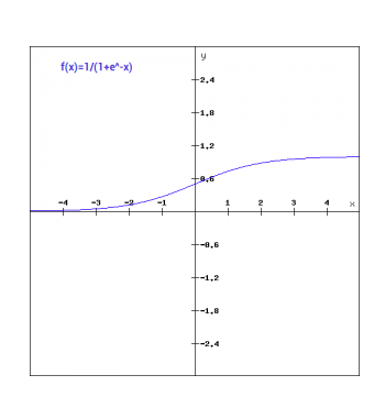
This results in a smooth gradient, with clear predictions. However, the outputs are not centered around 0, and it is computationally inefficient:

• The use of an exponent in the calculation can be slow over the thousands or millions of data points.
• They suffer from the “vanishing gradient” problem. The Sigmoid function sends large values to 1, and small values to 0, and is really only sensitive to changes around the midpoint (0.5). So, for very high or low values of \(x\), very little change in the prediction occurs, making it challenging for the learning algorithm to continue to adapt the weights to improve the performance of the model.

Tanh

The Tanh function is basically the same as the sigmoid, except shifted to the range of -1 to 1, calculated as follows:

\[(e^x – e^{-x}) / (e^x + e^{-x})\]

This has the benefit of centering the data around zero, making learning easier for future layers.

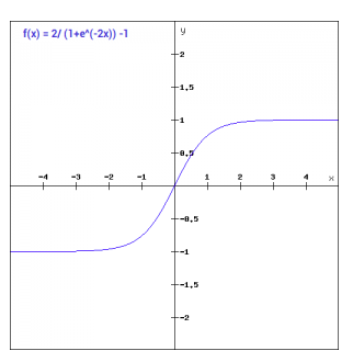
However, Tanh also suffers from the same efficiency problems as the sigmoid function.

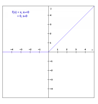
ReLU

The “rectified linear unit” activation function is a simple calculation that returns the value provided as input directly, or zero if the input is negative.

\[max(0, x)\]

ReLU has several advantages:

• It overcomes the vanishing gradient problem, since the function provides more sensitivity to the activation sum input and avoids easy saturation – the gradients remain proportional to the node activations.
• It is easy to implement, requiring only a max() function.
• It is capable of outputting a true zero value, unlike Tanh and Sigmoid which approximate a zero output with values close-to-but-not-exactly zero. When hidden layers contain true zeros this sparse representation can accelerate learning and simplify the model.
• It is good for cases where we don’t want the output to ever be negative (e.g. housing prices).

However, one must be wary of the (somewhat dramatically-named) Dying ReLU problem: If large weight updates result in the summed input to the activation always being negative, the node will always output zero, so the network cannot perform backprop and learn.

The Leaky ReLU attempts to overcome this by using a slight positive slope (a tunable hyperparameter) for negative values. The challenge with this is that the predictions are not consistent for negative input values.

Generally speaking, ReLU is the most-commonly used activation function for hidden units, particularly in MLP or CNN models, though RNNs still commonly use Tanh or Sigmoid. There are also plenty of other new and fancier options that can be explored if these more common activation functions prove unsuccessful (like Google’s Swish).

Activation Functions for Output Layers

The choice of activation function for the output layer depends on the prediction task.

Linear

Unlike in hidden layers, linear activation functions are used for output layers where the prediction is a regression task. It does not change the input in any way, and simply returns the value directly.

Sigmoid

The Sigmoid activation function is used for output layers in binary classification tasks, or multi-label tasks (using one node for each binary label).

Softmax

Softmax is used for multi-class classification. Softmax is related to the argmax function, which outputs 0 for all options that were not predicted, and 1 for the chosen option. Softmax instead allows for a probability-like vector of values that sum to 1, which can be interpreted as probabilities of class membership. It is calculated as:

\[e^x / sum(e^x)\]