Algorithms

5 minute read

What I Learned: Big O Notation and Sort and Search Algorithms

For the last few weeks I’ve been working through Harvard’s Intro to Computer Science course (CS50) online. It has been super helpful for understanding concepts that I’ve heard in passing before, but never really dug into.

This week’s topic was algorithms. Algorithms are essentially just a set of step-by-step instructions used to complete a particular task. The course focused on a few examples of algorithms used for searching and sorting, with a particular focus on comparing time complexity with Big O notation.

The O in Big O notation stands for “on the order of.” It represents a general approximation of how quickly runtime grows relative to some input, as that input gets to be arbitrarily large. It is general because it’s hard to pinpoint the exact runtime as this depends on things like the speed of the processor, or other processes taking place on the computer at the same time. It is relative based on the size of the input rather than being defined in absolute terms (like the number of seconds). The arbitrarily large input size is relevant for justifying our generalizations of runtime as constants become less significant.

The opposite of Big O notation is Big \(omega\), which refers to the best-case runtime. This is typically not as important as the worst or average case, however. As a side note, when \(O\) and \(omega\) are the same, we can denote this with \(theta\).

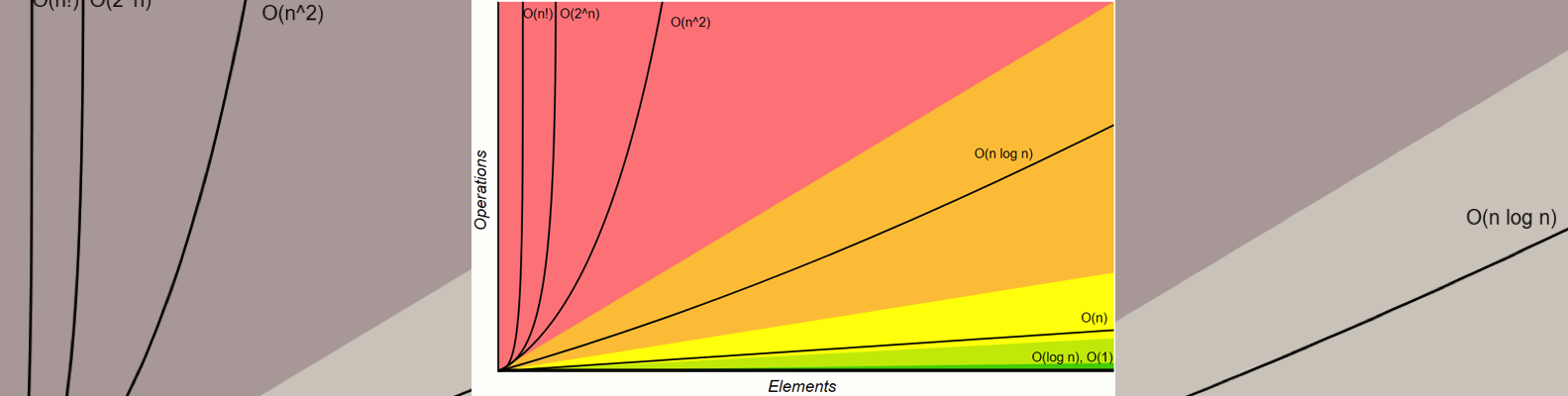
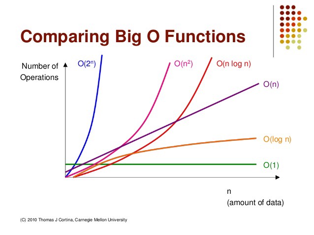
Some examples of Big O notation include:

\(O(1)\) or \(O(c)\). Constant time. The steps required to complete the execution of an algorithm remain constant, irrespective of the number of inputs. It doesn’t matter if we have 1 input or 1 million, it will always take just one “step.”
\(O(n)\). Linear time. The steps required to complete the execution of an algorithm increase or decrease linearly with the number of inputs. If we have \(n\) inputs, we will need \(n\) steps.
\(O(n^2)\). Quadratic time. The steps required to execute an algorithm are a quadratic function of the number of items in the input. This is particularly common when using nested iterations, such as executing something \(n\) times for \(n\) items.
\(O(log n)\). Logarithmic time. If we have a problem like binary search where we are halving a dataset, the growth curve peaks at the beginning and slowly flattens out as the size of the dataset increases - e.g. an input data set containing 10 items takes one second to complete, a data set containing 100 items takes two seconds, and a data set containing 1000 items will take three seconds.

There are many other common complexities, such as exponential and log linear.

image-center

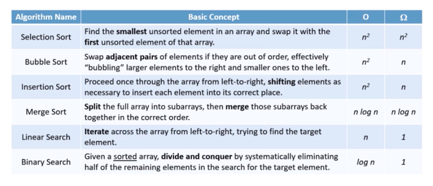
To illustrate, the course covered two search algorithms - linear search and binary search - and four sorting algorithms: selection, bubble, insertion, and merge sort.

Linear Search Let’s assume we are looking for a particular element in an array. With linear search, we simply search the array from left to right until we find the item we are looking for. In the best case, this is \(omega (1)\) if our desired element is the first one on the left. In the worst case, we will need to look through all of the elements of the array. So, linear search runs on \(O(n)\) time.

Binary Search The example that’s often used for binary search is that of looking for a name in a phone book. We might open the phone book in the middle, and see which page we are on. If the name is on the page we turn to, we’re done! If not, we see if the name is earlier or later in the alphabet. We then flip to halfway in the direction of the name, and repeat the process. In the best case we find the name right away on the first flip (\(omega (1)\)). Worst case, this process takes \(O(log n)\). However, a key consideration is that binary search requires that our data be sorted, which may also take time.

Bubble Sort With bubble sort, we look through the array and compare two adjacent elements. If the item on the right-hand-side is smaller than the left, we switch them. This slowly pushes larger elements to the right. In the best case, we would go through the array and not have to swap anything if it is already sorted (\(omega (n)\)). Worst case, this algorithm runs on \(O(n^2)\), which is quite slow for large data sets.

image-center

Selection Sort Selection sort involves iterating through each item in the array and locating the smallest element. When the smallest element is found it is brought to the front (the end of the sorted portion). Whatever element was originally in this position is switched with the index where the smallest element previously was. The process is repeated from the first unsorted index until all the elements have been sorted. This algorithm runs on \(theta(n^2)\), because in both the best and worst cases we are required to go through \(n\) elements \(n\) times, so this is another slow option.

image-center

Insertion Sort Insertion sort also iterates through an array to find the smallest element, but then rather than switching the smallest element with the first-unsorted element, it pushes the elements aside to make room for the new smallest element. This builds the array in place, and requires going forward through the array only once (though potentially back to make room for the new elements). The best case here is \(omega (n)\) if everything is already sorted, and \(O(n^2)\) if the array were to be in reverse order, necessitating shifting all the elements every time. Insertion sort works well for smaller lists.

image-center

Merge Sort Merge sort is the most (time) efficient of the presented algorithms. In this recursive approach, the data are halved repeatedly until each “half” is a series of 1 element arrays. These arrays are then merged back together starting with the smallest element, resulting in two-element arrays. Then, two-element arrays are merged and sorted, resulting in sorted four-element arrays, and so on. Merge sort runs on \(theta(n log n)\) time, because \(n\) elements are merged \(log n\) times. While more time efficient, merge sort may be more memory intensive.

image-center