Shapley values: From Game Theory to IML

What I Learned: All about Shapley values and implementing them for IML in Python!

For the last few months I’ve been working on designing a master’s thesis project for a student who will join us at INWT. The project centers on NLP and deep learning, with a core component being the explainability of predictions.

I have some experience with interpretable machine learning (IML) from my own master’s thesis, where I used LIME to evaluate predictions from a neural network classifier. Another option we’ve been considering employing for this project is SHAP/Shapley values, which I’ve heard about but haven’t really dug into yet.

It turns out that SHAP has its roots in game theory, and is based on a concept of Shapley values as developed by Lloyd Shapley in 1951. In general terms, game theory provides a theoretical framework for analyzing decisions among independent competing players in social situations. In a “game,” the “players” seek to optimize their personal results, which depend on the decisions of others as well as the players’ personal identities, preferences, and available strategies. Game theory maps these situations mathematically to determine the outcome given that the players behave in a rational way.

Lloyd Shapley focused on cooperative game theory, which assumes that “coalitions” of players are the primary decision-making units, and thus games are seen as a competition between different coalitions versus between individuals. In such a situation, a key consideration is how to fairly divvy up the costs and rewards across the actors in the coalition. Shapley values are an option for approaching this problem, and are particularly useful in situations where the contributions of actors to the final outcome are unequal. In other words, Shapley values help to determine the individual payoffs to all players where each player may have contributed more or less to the outcome.

So, what does this have to do with IML? Basically, with Shapley values we can quantify the contribution of each player to the game. With SHAP (SHapley Additive exPlanations, as originally proposed in this paper), we approach the problem of interpretability in a similar manner to determine the contribution of each feature to a prediction by the model we aim to explain.

We can calculate Shapley values by taking different “coalitions” of feature values and comparing their predicted outcomes to evaluate the influence of individual features. Since the number of possible coalitions grows exponentially, we take repeated samples and average them, so our Shapley values are estimates with some degree of uncertainty (which of course declines with more samples). In the end, we find the average marginal contribution of a feature value across all possible coalitions. Basically, we are trying to find the correct weight such that the sum of all Shapley values is the difference between the predictions and average value of the model. These final Shapley values correspond to the contribution of each feature towards pushing the prediction away from the expected value. Note that this is not the same as the difference in prediction if we were to remove the feature from the model!

Shapley values can be applied to both classification (where we are interested in probabilities) and regression, and on a global or local level. From a global perspective, Shapley values indicate how each feature contributed to the final prediction. Locally, Shapley values can help to analyze how the model made a decision for an individual data point. Another neat feature is that the local Shapley values sum to the model output, and global Shapley values sum to the overall model accuracy, so that they can be intuitively interpreted, independent of the specifics of the model.

Here are some examples. I’m using a custom news dataset that a classmate and I scraped from the politics sections of eight US news outlets from March - April 2020. We filtered for articles that contain references to either Joe Biden or Bernie Sanders, implemented BERT embeddings, and aimed to classify sentences that referenced each candidate (with the names removed of course) in a CNN. In this case I’m using the same dataset, except with one-hot encoding and a simple feedforward neural network.

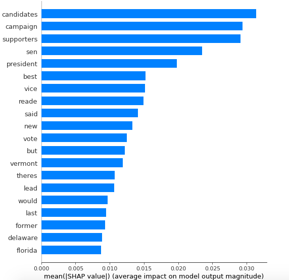
The model (without a lot of fussing or hyperparameter tuning) resulted in accuracy and F1 of 81%. Since that’s not the main focus for the project, it’s good enough for now! Using the shap.DeepExplainer, I first took a look at global variable importance:

These results seem quite logical - particularly words like Reade that are very specific to the dynamics of this particular campaign.

In this local example, the model predicted a value of 0.64, where sentences labelled 0 reference Biden, and those labelled 1 reference Sanders. The absence of the words “primary”, “president”, “candidates”, and “win” influenced a higher prediction that this sentence referenced Sanders. The lack of “would” and “supporters,” and the inclusion of the word “campaign” led to a lower predicted probability that the sentence referenced Sanders.

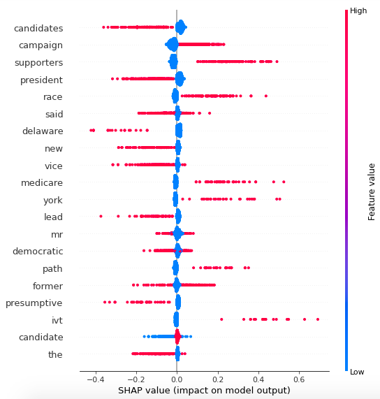
SHAP can also create this cool summary plot:

Here, variables are listed in descending order in terms of importance, and the horizontal location shows whether the effect of that value is associated with a higher or lower prediction. The color bar on the right-hand side shows that red is associated with higher values (1 in our case) and blue with low values (0). So, for example, we can see that having 1 in “campaign” (basically, if the sentence contained the word campaign) is strongly associated with Biden, while a 1 on “supporters” is strongly associated with Sanders.

There’s still a ton more for me to learn on this topic, but this was a fun introduction! All the code for this project is available here.