Bayes Basics

What I Learned: The Basics of Bayesian Inference, MCMC, and Stan

One of my projects at INWT at the moment relies on Bayesian modeling for A/B testing. I’ve spent the last few weeks working through the course Statistical Rethinking which covers an introduction to Bayesian methods and Stan. Below I’ve summarized:

• The intuition behind Bayesian inference, and how it differs from more traditional frequentist methods
• Why one may choose to use a Bayesian approach
• The basics of Bayesian inference
• Markov chain Monte Carlo
• Stan for modeling

What is Bayesian Inference?

Essentially, Bayesian inference uses probability to define uncertainty. It extends the binary logic of something being true or false to continuous plausibilities. With Bayesian methods, we are able to incorporate our prior beliefs about an event into the model, and update our model based on new data.

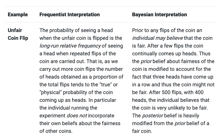
This is in contrast to “classical” or “frequentist” statistics, which instead assert that probabilities are simply the long-run frequency of random events over repeated trials. Frequentists focus on fixed parameters, with the goal being to minimize the uncertainty of estimates (which is caused by sampling variation). Confidence intervals are reported in terms of repeated sampling: For example, a frequentist might say, “Ninety-five percent of similarly-sized intervals in repeated samples will contain the population parameter.”

In contrast, Bayesian approaches consider uncertainty “internal,” and preserve and adjust it in light of new evidence. An example of internal uncertainty may be the outcome of a coin flip, which is generally considered to be random; The Bayesian approach would instead say that the outcome isn’t random at all - rather, that it is a deterministic process and we are simply ignorant (or uncertain) of the exact velocity and physics we would need to know to model the outcome. Therefore, the focus is on subjective probability, with the goal to estimate the statistician’s uncertainty rather than a fixed, constant parameter. Instead of confidence intervals, the Bayesian alternative is a “credible” interval. An example may be, “There is a 95% chance that the parameter exists within this interval,” which for many is a much more intuitive interpretation.

Interestingly, Bayesian inference is actually the “original” version of statistics, and traditional techniques like linear regression actually started as a Bayesian procedure. However, Bayesian approaches can be computationally heavy, so it wasn’t until computing power expanded that they became widely used again.

Bayesian estimates are made by counting all the ways the data we see could have arisen, according to our assumptions, and ranking all of these ways relative to each other. The idea is that assumptions that can arise in more ways are more plausible.

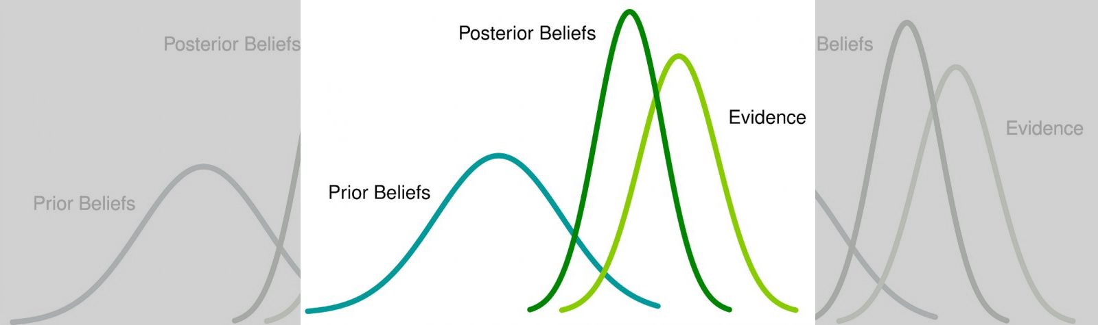
In this context, “assumptions” references the statistician’s prior beliefs. This is the knowledge they have before the test: For example, the distribution of a website’s average conversion rate. Without any prior knowledge, this could be represented as a “flat prior,” where the prior distribution takes the form of a uniform probability distribution from 0 to 1, meaning that before seeing any data, the model assumes that any conversion rate between 0 and 1 (0% to 100%) is equally likely. Once we see new data, our knowledge about the true relationship is updated, which is incorporated to create the posterior distribution. This posterior can be used to make statistical calculations, and/or serve as a prior for the next round.

This example from this blog illustrates these concepts quite well, and contrasts them to a frequentist approach:

Why Use Bayesian Methods?

Bayesian methods tend to be more computationally challenging to implement than frequentist approaches. However, they have many advantages, including:

• Interpretability: Unlike frequentist approaches that use metrics such as the p-value to make test decisions, Bayesian methods are able to give the probability that A is better or worse than B.
• Test sample size is much less relevant, so test decisions can be made more quickly.
• Alpha-adjustement is not necessary. Unlike with frequentist statistics, where alpha-adjustment is needed when more than one analysis is done on the same data, one can conduct multiple analyses on a data set and draw resulting inferences without risking increased likelihood of false conclusions.

Notably, with large sample sizes prior knowledge becomes less relevant and Bayesian and Frequentist inference eventually converge to the same anyway.

How does Bayesian inference work?

Statistical Rethinking begins with a simple example to illustrate the application of Bayesian methods, called the Garden of Forking Data, which I’ve summarized here.

Let’s say we have a bag containing four marbles. We know the marbles may be blue or white, but we don’t know how many marbles of each color are in the bag (if any are at all). If we make three draws from the bag with replacement, and end up drawing blue, white, blue, we can look at each possible combination of marbles to see the plausibility of the true distribution in the bag resulting in the data we have observed.

Since we have drawn both blue and white marbles, we know there can’t be four white or four blue marbles. So, let’s look a the first possible combination: one blue and three white.

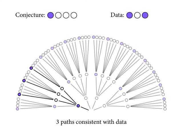
Starting from the middle and moving outwards, there are three possible ways the data we’ve observed (drawing blue, then white, then blue) could have happened, if the true distribution of marbles in the bag were one blue and three white.

We can repeat this for the other possible marble distributions.

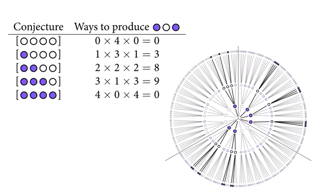
At the end of this process, we can see that three blue and one white has the highest count. But if we get more data, we can update our beliefs. If we draw another blue marble, we add a layer to the garden of forking data, and multiply the previous counts by the number of ways we could draw a blue marble on the fourth draw.

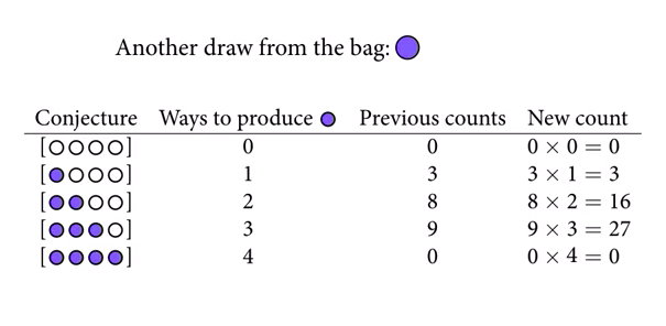
Now, three blue and one white is looking even more plausible. Note that the absolute counts aren’t important, just the relative plausibilities. These counts can be converted to probabilities by dividing each count by the sum of all counts.

Bayesian methods also naturally accommodate using different kinds of information to update posterior beliefs. For example, let’s say the marble factory tells us that blue marbles are rare, but that all bags contain at least one blue marble. They also give us the factory count of different bags with different marble distributions.

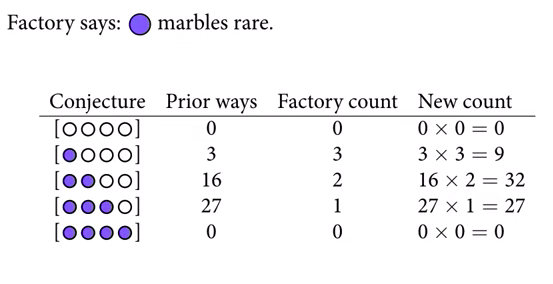
The posterior distribution is simply the product of the prior and the probability of the data.

Bayes’ Theorem formalizes the relationship from the garden of forking data.

\[P(A \mid B) = \frac{P(B \mid A) \, P(A)}{P(B)}\]

\(P(A \mid B)\) is the posterior - our updated belief about \(A\) once the evidence \(B\) has been taken into account. To use the coin toss example, this is our updated belief about the fairness of the coin, after seeing some number of flips.

\(P(B \mid A)\) is the likelihood - the probability of observing the data, given the parameter \(theta\) taking different values. If we knew the coin was fair, this gives the probability of seeing \(x\) heads in \(n\) flips.

\(P(A)\) is the prior - our beliefs about \(A\) before seeing the data \(B\). Our prior beliefs about the fairness of the coin, before flipping it at all.

\(P(B)\) is the evidence - the average probability of the data given all possible values of \(A\). If we had many views of the fairness of the coin, but were not certain which was accurate, the evidence tells us the probability of seeing a certain sequence of flips for all possibilities of our beliefs about the coin’s fairness. This value is important as it is the “normalizing constant” that ensures the posterior distribution integrates to 1 (i.e. all probabilities sum to 1).

If we are not concerned about scale, we can drop the normalizing constant and instead asserting simply just that

\(P(A \mid B)\) is proportional to \(P(B \mid A) * P(A)\)

A good visual example of how the posterior is calculated using Bayes’ Theorem can be found at minute 10:45 of this video.

Another simple example could be: Imagine it rains one out of every 10 days, and that 50% of all rainy days start off cloudy in the morning. Four out of 10 days it is cloudy, though. What is the chance of rain today, given that it is cloudy this morning?

\(P(rain \mid cloudy) = P(cloudy \mid rain) * P(rain) / P(cloudy)\) \(P(rain \mid cloudy) = 0.5 * 0.1 / 0.4\) = 12.5%

In practice, posteriors are typically not point estimates, but rather estimated distributions. These distributions can then be sampled from (with replacement) to generate statistics. For example, the textbook for Statistical Rethinking suggests some common questions:

• How much posterior probability lies below some parameter value?
• How much posterior probability lies between two parameter values?
• Which parameter value marks the lower 5% of the posterior probability?
• Which range of parameter values contains 90% of the posterior probability?
• Which parameter value has the highest posterior probability?

As a concrete example, say you wanted to estimate a regression coefficient: Since a Bayesian analysis will result in many values from the distribution for that coefficient, you must first estimate the posterior and then use it to estimate the mean, or a credible interval.

It is also typically challenging to calculate the joint posterior distribution in a multivariate, complex model, which may not have pretty distributions. For this reason techniques like Markov chain Monte Carlo are typically employed.

Markov chain Monte Carlo

When it isn’t possible to compute the posterior distribution directly, we can approximate it using techniques like Markov chain Monte Carlo (MCMC). There are a variety of specific MCMC algorithms, all of which draw samples from the posterior, resulting in a collection of parameter values. The frequencies of these values correspond to the posterior plausibilities. You can then build a picture of the posterior from the histogram of these samples.

The intuition behind how MCMC methods work is illustrated by decomposing the name:

• Monte Carlo sampling estimates a distribution by examining random independent samples taken from it. Monte Carlo estimation doesn’t work well in high-dimensions.
• Markov chains are sequences of events that are probabilistically related to one another. Each event comes from a set of outcomes, and is determined by the previous event based on a fixed set of probabilities. This allows the algorithm to more quickly narrow in on the approximated distribution even with large numbers of variables. Markov chains have the “Markov Property,” which means that the next state only depends on the most recent state, and not those before it.

So, MCMC allows random sampling of high-dimensional probability distributions, where each sample is used as a “stepping stone” to generate the next sample.

The next step is suggested, and then the algorithm decides whether or not to go there based on some acceptance-rejection criteria. There are two main families of acceptance-rejections algorithms: those descended from the Metropolis algorithm, and Hamiltonian Monte Carlo.

Metropolis algorithms are “guess and check.” We begin at a point, make a guess for the next step, check the posterior probability at that location, and based on a comparison between the current and proposed point, either move or don’t. The quality of the proposals is critical, because it’s easy to get stuck in one area.

Hamiltonian Monte Carlo, on the other hand, is more involved. It represents the current point as a particle and runs a physics simulation, whereby the particle is “flicked” in a random direction. The curvature of the distribution is taken into account, resulting in a more efficient algorithm with better proposals.

In general, MCMC algorithms are sensitive to their starting point, and require a “burn-in” phase for the model to figure out the search space a bit. These initial warm-up samples are then discarded. The number of samples required depends on the goal - something simple like the posterior mean may get by with only 200 samples, whereas a 99% credible interval estimate may need many more. It’s possible to estimate more than one chain: the Statistical Rethinking course recommends one for debugging, and four for inference.

Side note: Conjugate Priors

A conjugate prior is when the prior retains its parametric form through to the posterior, making the estimation much simpler mathematically. Since we can choose our priors, we may choose to work with conjugate priors for convenience.

Likelihood > Conjugate prior

1. Normal > Normal
2. Binomial/Bernoulli > Beta
3. Exponential/Poisson > Gamma
4. Uniform > Pareto
5. Multinomial > Dirichlet

This is something for me to look deeper into in the future!

Bayesian modeling with Stan

Ok, so how do we actually build a Bayesian model?

The Statistical Rethinking class has a companion package called rethinking that allows for the specification of models with a simplified interface. It uses Stan under the hood, which is the software that is most commonly used for Bayesian modeling. Stan can be accessed through R, Python, and many other languages, and uses its own syntax that is similar to C++.

A Stan script begins with a “data block,” where we tell Stan the data it should be expecting from the data list. This can be followed by a “transformed data block” if any transformations (e.g. log) are needed. Next, the parameters are specified (and optionally transformed), and finally the model is specified. This is where the priors and likelihood are noted, along with the declaration of any necessary variables.

Here’s a basic example. We first specify our Stan model:

data {

	int N; // sample size
	real Y[N]; // array of continuous values 
}

parameters {

	real mu;
	real<lower=0> sigma; // sigma constrained to be non-negative

}

model {
	
	for(i in 1:N)				// for loop defining likelihood
		Y[i] ~ normal(mu, sigma); 	// for each observation

	mu ~ normal(1.7, 0.3);			// prior for mu
	sigma ~ cauchy(0, 1);			// prior for sigma

}

(I must say, I’m grateful that I already had a bit of C knowledge from CS50 before digging into this!)

Then, in R, we generate some fake data, fit the model, and explore the results.

# generate data
N <- 1000 # sample size
Y <- rnorm(N, 1.6, 0.3) 

# compile model
library(rstan)

model <- stan_model('stan_model.stan')

# pass data to stan
# must use named list, specify iterations and chains
# can also use parallelism here
fit <- sampling(model, list(N = N, Y = Y), iter = 200, chains = 4)

# diagnose 
print(fit) # summary stats for each parameter

# graph
params <- extract(fit) # extract posterior samples
hist(params$mu) 

# fancy diagnostics
library(shinystan)
launch_shinystan(fit)

Good overviews of using Stan can be found here and here. This YouTube tutorial is also helpful.

As an aside, if Stan is ever tricky, it’s possible to create the model in the rethinking package and then use stancode(model) to get the Stan code itself.