Mathematics for Machine Learning: Calculus

I’ve been having a really good time going back and learning about/reviewing the mathematical fundamentals for machine learning recently. Over the holidays I spent some time working through Imperial College London’s Multivariate Calculus course on Coursera, as well as 3blue1brown’s Essence of Calculus series (which is amazing, like all of his work). All of the black background images below are from the 3blue1brown videos.

I’m putting together this blog to review the content and make sure I really understand it, as well as to prepare some notes for the future. I will not include anything on doing calculations by hand, though this did feature quite heavily in the Coursera course.

What is Calculus?

Basically, calculus is a set of tools to describe the relationship between a function and a change in its variables. The key concept is quantifying change. Calculus is the core of many applications in machine learning, such as gradient descent and neural networks.

Many tough problems in math and science can be broken down and approximated as the sum of many small quantities. For example, we might be curious about the velocity function of a car over some distance traveled, measured at several small time intervals. Or, we might want to figure out how to measure the area of a circle by slicing it up into thin concentric rings, and adding them together.

If finer and finer approximations of the original problem (i.e. shorter time periods for the car example, thinner rings for the circle problem) correspond to smaller and smaller “rectangles”, then the original problem is equivalent to finding the area under some graph.

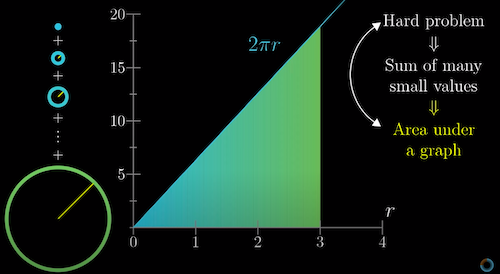
Solving such a problem is quite simple in the linear case, but can also be extended to non-linear gradients that change with different input values in a function.

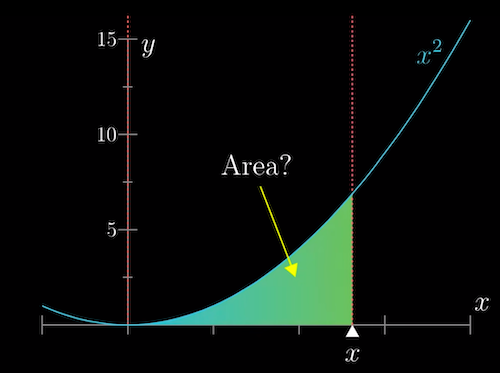
Two fundamental concepts in calculus are derivatives and integrals. Differential calculus essentially cuts a graph into small pieces to find how it changes. Integral calculus joins the small pieces together to find the area under the graph.

Derivatives

Derivatives are a measure of how sensitive a function is to small changes in its input. It is an approximation for the slope around a given point.

But, how do we find the slope of a function at a single point? We might simply choose a nearby point to the point in question, and approximate the slope between them. For smaller and smaller differences between the points, this approximation gets better and better. This is the derivative.

Derivatives of the function \(f(x)\) would be denoted as either \(f’\) or \({\frac{df}{dx}}\). The basic formula is:

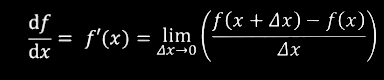
Where \(\Delta x\) is the tiny nudge to \(x\).

Once we differentiate a function, the result is a new function. If we differentiate the resulting function again, we call this the second order derivative. Differentiating once more results in the third order derivative, and so on.

We can also think about antiderivatives: Essentially, if we wanted to find the antiderivative \(f(x)\) for some function \(f'(x)\), we’d ask ourselves what function we’d need to differentiate to get \(f'(x).\)

Derivative Rules

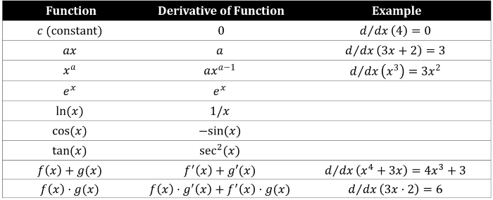
There are a few time-saving rules that are helpful for quickly calculating derivatives. Others exist, but some of the most fundamental are:

• Power rule - If we have a function with a power, the exponent “hops” down in front, leaving one less of itself: \(x^3\) becomes \(3x^2\).
• Sum rule - We can simply differentiate each term separately and then add them together again: \(x^4 + 3x\) becomes \(4x^3 + 3\).
• Product rule - If two functions are multiplied, we first multiply the first original function with the derivative of the second, and then the second original function with the derivative of the first, and add them together. A good mnemonic device for this one is (sing-songy) left d-right, right d-left. \(A(x) = f(x)g(x)\) becomes \(A’(x) = f(x)g’(x) + g(x)+f’(x)\). For more than two functions, the process is the same, except that each time only one function in the multiplication is the derivative, while the others are the originals, and all are added back together.
• Chain-rule - If we have nested functions such as \(h(x) = f(g(x))\), the derivative of the outside function is evaluated with the original inside function, multiplied by the derivative of the inside function: \(h’(x) = f’(g(x)) * g’(x)\).

There are also some interesting relationships that always hold. For example:

• The derivative of a constant (for example, 5, or 0) is 0.
• The derivative of \(e^x\) is always \(e^x\), even at the second, third, etc. order.

This useful chart covers several of the above, as well as some trigonometry functions that are common in calculus:

Partial Derivatives

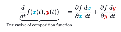
If we have a function that takes in more than one variable, we can differentiate with respect to each one individually, holding the others constant, and find the total derivative using the multivariable version of the chain rule.

For example, given a multivariable function \(f(x, y)\) and two single variable functions \(x(t)\) and \(y(t)\), we can calculate the total derivative as follows:

Integrals

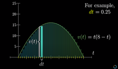
Integrals are essentially the inverse of derivatives. To illustrate, imagine that you’re in a car, and you can only see the speedometer at different points in time. Given only this information, how can you estimate the total distance traveled over some length of time?

If the car traveled a constant speed which changed abruptly at discrete points in time, this would be easy. We can approximate the car’s true constantly-changing velocity using smaller and smaller time intervals to arrive at a more precise answer. If we add up all of these tiny approximations, we’d get the total distance traveled. This is the integral.

Jacobian

If we have a function of many variables \(f(x1, x2, x3, ...)\), then the Jacobian is simply a vector where each entry is the partial derivative of \(f\) with respect to each one of those variables in turn. In other words, it is a vector of the first-order derivatives for each variable in our function of interest.

Jacobians are typically written as row vectors. Jacobians for several functions can also be stacked on top of one another to form a matrix.

The Jacobian is an algebraic expression for a vector, which, when we plug in specific values for the coordinates, will return a vector pointing in the direction of steepest uphill slope for this function. The steeper the slope, the greater the magnitude of the Jacobian at that point. This can be used to find the minimum or maximum of a function.

Hessian

The Hessian is a matrix of second-order derivatives, which can be calculated by differentiating the terms in the Jacobian again.

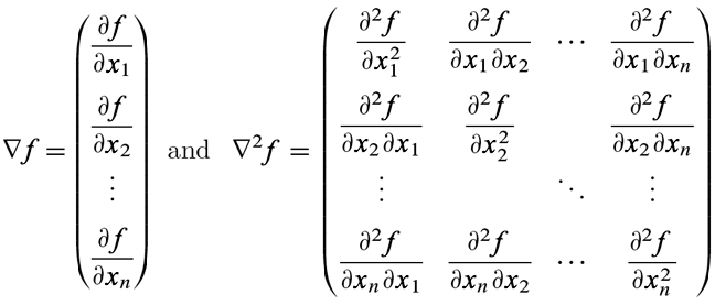
Hessians are symmetrical across the leading diagonal, assuming the function is continuous.

While the Jacobian can be used to figure out whether we’re dealing with a maximum or a minimum, it doesn’t robustly determine which we have found. This is where the Hessian can help:

• If the determinant of a Hessian is positive, we know we’re dealing with either a maximum or or minimum. We then just look at the first term in the top left, and if it is positive we know we have a minimum, while a negative first term indicates a maximum.
• A negative determinant means we are not at a maximum or minimum. However, we could have a negative determinant with zero gradient, which would indicate a saddle-shaped function.

Taylor Series

A Taylor Series can be used to approximate complex functions using a power series. This allows us to reduce computational complexity, and the use of polynomials makes the function easier to differentiate, integrate, and perform additional calculations on. While this only works for functions that are continuous and can be differentiated as many times as desired, many applications in ML are well-behaved, so this approach can be quite useful.

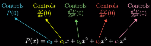
\[f(x) = a + bx + cx^2 + dx^3 + …\]

In the above, \(a\) is the zeroth order approximation, \(b\) is the first order, etc. \(a\), \(b\), \(c\), \(d\), and so on, are constants that we adjust to fit the original function.

In the univariate case, the process to calculate a Taylor Series is the following:

• Pick a starting point on the function curve. In a Maclaurin Series, this is always 0. The Taylor Series acknowledges that there is nothing special about the point \(x = 0\), so rather expands to say that if we know everything about a function at any point, we can reconstruct the function anywhere.
• The zeroth order approximation is the intercept, or the point \(f(x)\).
• First order approximation can have a gradient, so we take the first derivative evaluated at the starting point.
• The second order approximation can curve the line from the first order approximation, so we take the second order derivative.
• And so on, through to as many orders as needed to satisfactorily approximate the function.

In the example below, the function is \(P(x)\) is approximated at \(x=0\).

An interesting note is that earlier orders are not affected by later ones. Once we’ve taken the first order derivative and assigned that to the coefficient, it doesn’t change based on the values of later coefficients. In other words, once we pick the first order, we are free to change the second order to continue improving the match to the function, and the first order will always remain the same.

In a Maclaurin series, this is because we’re working with the point where \(x = 0\), so the \(x\) terms cancel out. In a Taylor Series, we simulate this effect by subtracting the starting value from \(x\):

\[P_z (x) = a + b(x - z) + c(x - z)^2 + d(x - z)^3 + …\]

Because the terms in a Taylor Series are polynomials, when we take the derivatives we’re going to end up having to work with the power rule. So, ultimately we divide the derivative by the factorial of the power to cancel out the power effect.

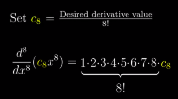
Thus, the final formula is:

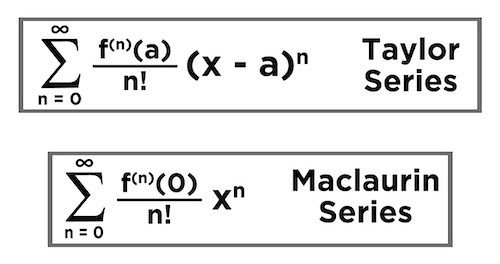
The Taylor Series can also be expanded to the multivariable case.

Newton-Raphson

The Newton-Raphson method can be used to find the roots of univariate functions. The process is fairly simple:

• Pick an initial value for \(x\). Evaluate the equation to get the value of \(y\) and the derivative at that point.
• Use the derivative to “point” to the next guess for \(x\). Visually, we can think of the tangent of the derivative and where it intersects with the x-axis. Numerically, the next guess is chosen using the equation:

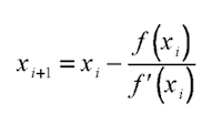
• Continue the process until the value of \(x\) converges close enough to \(y\). Some important notes are that sometimes derivatives may point back and forth in a loop between a few estimates for \(x\). Convergence is also slower when close to a maximum or minimum, since the slope is less extreme.

Basic Gradient Descent

Gradient descent is intuitively quite similar to the above, except it can be used in the multivariable case.

Now, when considering how to find the optimal values for the variables such that a cost function is minimized, rather than the slope we need to think about which direction in a multi-dimensional space we should “step” to decrease the output of the function most quickly. In other words, what is the steepest downhill direction?

A key concept is Grad, denoted \(\triangledown\). It is a vector of the first-order derivatives for each variable in a function. It gives the direction of steepest ascent. Taking the negative of the gradient gives the direction to step to decrease the function most quickly. Moreover, the length of this gradient vector is an indication of how steep the steepest slope is.

If we want to know how much the function will change when we move along some unit vector in an arbitrary direction, we can take the dot product of this vector with Grad.

The formula is similar to that for Newton-Raphson. Starting at some point \(s_0\), we take some step downhill \(\gamma\), multiplied by the Grad of \(f\), evaluated at \(s_0\):

\[s_1 = s_0 - \gamma \triangledown f(s_0)\]

We continually reevaluate, based on some learning rate (which determines the step sizes/how much the coefficients change on each iteration), until we find a minimum. A large learning rate may cause us to miss the minimum, while a small learning rate results in slower training time.

Of course, it is possible to only find a local minimum. Stochastic gradient descent may be a solution to this, whereby instead of taking a step by computing the gradient of the loss function created by summing all the loss functions, we take a step by computing the gradient of the loss of only one randomly sampled (without replacement) example. This wasn’t covered in the course, and though I am already somewhat familiar with the topic, I want to look into this in more detail in the future.