Back to Basics: Interpreting Logistic Regression

Logistic regression is one of the most foundational statistical models, and also one of the most frequently misinterpreted. Which is fair, because odds-ratios aren’t exactly intuitive at first. What follows is an overview of the fundamentals of logistic regression, and how to properly interpret the model output.

What is logistic regression?

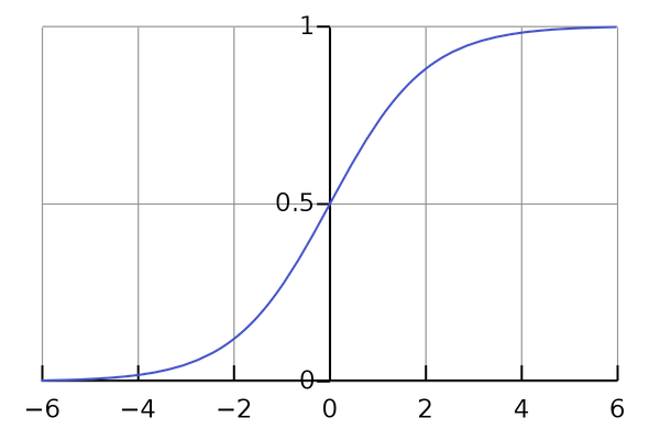
Logistic regression models the probability that an observation belongs to one of two classes, though it can also be extended to multinomial or ordinal outcomes. We use logistic regression instead of linear regression because linear regression is unbounded, meaning it can predict values more extreme than 1 and 0, while logistic regression uses the logistic function (sigmoid) to constrain the values within that range.

How is logistic regression estimated?

In logistic regression, the y-axis is transformed from probability to log odds using the logit function: \(log(p / 1 - p)\).

Even though we associate logistic regression with the sigmoid, once we use the logit function the coefficients are represented as a straight line on the log odds graph, where a probability of 0 is negative infinity, a probability of 0.5 is 0, and a probability of 1 is infinity. Because of this transformation, the residuals are infinity, so we can’t use OLS to calculate the values of the coefficients.

Instead, coefficients are typically estimated using maximum likelihood (MLE). The goal of MLE is to find the optimal way to fit a distribution to the data we have: In other words, we choose a distribution and parameters such that they maximize the likelihood of observing the data we observe.

The process of estimating coefficients using MLE is:

• Transform log odds to probabilities.
• Calculate the log likelihood given these probabilities and a hypothetical line.
• Choose a line that maximizes the log likelihood.

It is also possible to use gradient descent as an alternative method to calculate the coefficients. Gradient descent is an optimization algorithm used to find the best values for coefficients such that a cost function is minimized. This is done by iteratively moving in the direction of steepest descent, as defined by the negative of the gradient. The goal is to try different values for the coefficients, evaluate their cost, and select new coefficients that have a slightly lower cost. Repeating this process enough times will lead to the bottom of the cost function – where the slope is 0 – and the values of the coefficients result in the minimum cost.

Logistic Regression Assumptions

Lots of the linear regression assumptions do not apply:

• Logistic regression does not require a linear relationship between the dependent and independent variables.
• The residuals do not need to be normally distributed.
• Homoscedasticity is not required.

The logistic regression does assume:

• There is minimal or no multicollinearity among the independent variables.
• There is a linear relationship between the logit of the outcome and each predictor variable.
• A binary outcome variable (obviously).
• Observations are independent of each other.

Odds vs. Probabilities

Understanding the distinction between odds and probabilities is critical to grasping logistic regression.

• Probability is the ratio of something happening to everything that could happen. For example, in the sports context, the probability of the team winning could be described as \(p(teamWinning)/p(teamLosing \text{ or } teamWinning)\)
• Odds are the ratio of something happening to it not happening, and can be calculated either from counts or probabilities. For example, \(p(teamWinning)/p(teamLosing)\).

To illustrate further, if the probability of an event is 0.8, the odds of the event occurring are 0.8/0.2 = 4. This says that the event will occur four times for every time the event does not occur, and this event has 300% higher odds of happening than not happening.

If the odds are against my team winning, they will be between 0 and 1, while if they are for my team winning then they go from 1 to infinity. This asymmetry makes it difficult to compare odds for or against my team winning. Taking the log of the odds solves this problem by making everything symmetrical and converting to a format that can easily be analyzed using a normal distribution. To convert odds to probabilities, the formula is simply \(odds / (1 + odds)\).

The relationship between odds and probabilities can be a bit tricky, so here are some more examples:

• A proportion of 50% corresponds to an odds ratio of 1/1, since there is one loss for each win.
• A proportion of 33%, on the other hand, corresponds to an odds ratio of 1/2 (two losses every one win).
• A proportion of 75% corresponds to an odds ratio of 3/1, etc.

Interpreting Model Output

Ok, so now that we have all that background out of the way, how do we actually interpret the results of a logistic regression model?

This simple overview won’t go in depth on every element, but intends to only serve as an easy-to-remember summary.

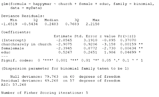
Deviance residuals

While we do have residuals in logistic regression, they aren’t very useful since they don’t come from some sort of principle of least-squares minimization. Because we fit logistic regression with MLE, it’s better to look at something that considers the log-likelihood function.

The deviance residual associated with an observation is the observation’s value evaluated under the log likelihood function, multiplied by -2. It essentially measures how well an observation fits the model (the closer to zero, the better the fit of the observation).

Deviance residuals should have properties similar to “normal” residuals. For example, we would be looking for them to be relatively symmetrical and centered around zero.

Coefficients

This is where things get…fun!

• The intercept is the log(odds) of the outcome when all the independent variables are 0.
• Continuous coefficients are the increase in the log(odds) for every one unit increase in \(X\), holding the other coefficients constant. If we exponentiate this, we get an odds-ratio for an increase of one unit. To convert to probabilities, we use \(exp(coef)/(1 + exp(coef))\).
  • But be careful here! The relationship between odds and probabilities is non-linear, and depends on the starting point. For example, 3% lower odds of passing a test is the same whether the test score is low, medium, or high. The difference in the probability of passing is not the same at those test scores, though: it’s bigger in the middle than at the ends because the relationship between the test score and the probability of passing isn’t linear, it’s sigmoidal, since increasing a test score by say, 2 points, has a very small effect for people whose scores are very low or very high, and a much larger effect for people whose scores are in the middle.
  • We can make predicted probabilities more intuitive by plugging in some plausible values for \(X\), and plotting them to see how the probabilities change with different values for the independent variables.
  • Alternatively, we can calculate risk ratios (RR), which are probability ratios: \(OR / (1 – p + (p x OR))\) where \(p\) is the risk in the control group. A RR of 3 means the risk of an outcome is increased threefold. A RR of 0.5 means the risk is cut in half. But an OR of 3 doesn’t mean the risk is threefold; rather the odds are threefold greater. The OR will always be an overestimate compared to the RR. The RR and OR will be similar for rare outcomes, < 10%. But the OR increasingly overestimates RR as outcomes exceed 10%.
• Categorical coefficients are the log(odds ratio) of a reference and comparison category (e.g. reference is female observations, comparison is male). This says, on the log scale, how much being in the comparison class increases or decreases the odds of the outcome relative to the reference category. For example, if we exponentiate an odds ratio with men as the comparison and women as the reference category, and get 2.04, we can say that men have 104% higher odds of an outcome than women do.
• Interaction terms can also be kind of tricky, and the interpretation depends on the type of interaction:
  • Two categorical variables: The difference between two log-odds ratios.
  • One continuous, one categorical: The difference between the log-odds ratios for two homogenous groups that differ only by one unit (for example, men and women ages 20 and 21).
  • Two continuous: The difference in the log-odds ratios for two groups, each of which differs by one unit (for example, grade level 10 and grade level 11, and age 20 and age 21).
• The Z-score is the coefficient divided by the standard error, or how far away it is from zero in the standard normal curve.
• The p-value is determined by the Wald’s test (in R at least). It determines if the comparison category is statistically significantly different from the reference category. An important note about p-values in logistic regression is that they are dependent on what is used as the reference category, and may change if this is adjusted in the model.

This lecture has some useful information on much of the above.

Null Deviance and Residual Deviance

Null deviance shows how well the response is predicted by the model with nothing but an intercept. A low null deviance implies that the data can be modeled well merely using the intercept (mean).

Residual deviance shows how well the response is predicted by the model when the predictors are included. A low residual deviance implies that the model you have trained is appropriate. For a well-fitting model, the residual deviance should be close to the degrees of freedom.

Null deviance and residual deviance are chi-squared statistics, and p-values for each can be calculated using the degrees of freedom. Comparing the difference between them allows for an examination of whether the deviance is the same between the two models.

They can also be used to compute pseudo R2 (\(residualDeviance/nullDeviance\)).

AIC

Residual deviance adjusted for the number of parameters in the model. It is used for comparing models, with a lower AIC value being preferable.