
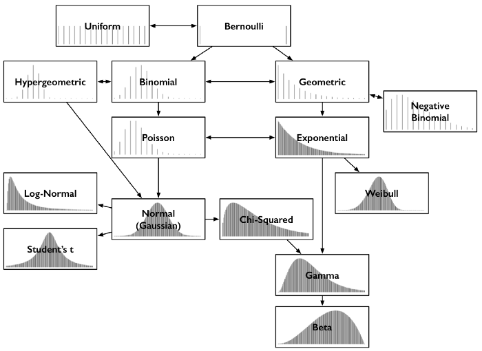
Common Probability Distributions
What I Learned: Getting Clear on Probability Distributions
Throughout my time working in quantitative methods, probability distributions have - of course - come up frequently. The very common ones are all clear in my head - but what about the distributions that I rarely work with? Since diving deeper into Bayesian methods these have been coming up more frequently, so I thought it would be worthwhile to spend a little bit of time reviewing the intuition behind 15 of the more common distributions.
Discrete Outcomes
Bernoulli
In a Bernoulli distribution there is only a single trial with two possible outcomes: 1 (success) or 0 (failure). The probability of success is the same in each trial, and is independent of all other trials.
If a random variable \(X\) has a Bernoulli distribution it will take the value 1 with the probability of success, \(p\), and the value 0 with the probability of failure, \(1 - p\). The probabilities for success and failure do not need to be equally likely. For example, imagine a single toss of a (possibly unfair) coin.
Uniform
The uniform distribution is characterized by a flat probability density function (PDF) - all outcomes are equally likely. For example, when rolling a fair die, the outcomes of rolling one through six are equally likely over an unlimited number of events.
Binomial
Like the Bernoulli distribution, there are only two potential outcomes from each trial: success or failure, and the probability of success is the same for each independent trial. Unlike a Bernoulli trial, binomial distributions consider experiments over \(n\) repeated trials (not just one).
Binomial distributions can be thought of as the sum of the outcomes of events that follow a Bernoulli distribution; For example, if a coin is tossed 10 times, how many times did it come up heads? This count follows a binomial distribution. Its parameters are the number of trials \(n\), and the probability of success \(p\).
Geometric
If the binomial distribution answers the question of how many successes there were, the geometric distribution answers the question of how many failures there were until a success. For example, how many times does a flipped coin come up tails before it comes up heads? It is also parameterized by \(p\), the probability of that final success, but not by \(n\), the number of trials, since this is a part of the outcome itself.
As a concrete example, with a fair coin there is a 50% chance that the first success will occur on the first flip, a 25% chance that it will occur on the second flip, and a 12.5% chance that it will occur on the third flip. The curve flattens out as the probability decreases, but will always be right-skewed.
Negative Binomial
The negative binomial distribution is similar to the geometric, except that it considers the number of failures until \(r\) successes have occurred, not just one.
Hypergeometric
A commonly-used example for a binomial distribution is the concept of drawing marbles out of a jar that has two kinds of marbles (let’s say half black and half white), with replacement. With replacement means that once we pick up a marble, we put it back in before picking up the next one, so the probability of picking a black or white marble doesn’t change.
But, what if we drew marbles without replacement? The probability of success would change over time as more marbles are removed, which would be especially pronounced if we started with few marbles in the jar.
This is an example of the hypergeometric distribution. It measures the probability of a specified number of successes in \(n\) trials, without replacement, from a finite population. The probabilities change as a function of the previous draws.
Poisson
Unlike the previous distributions, the Poisson distribution is parameterized not by the probability \(p\) and the number of trials \(n\), but rather the average number of events in a given time period. Put another way, rather than the probability that an event occurs, we are concerned with the rate at which an event occurs, parameterized by \(\lambda\).
Events are still assumed to be independent from one another, and the average rate between events occurring is constant. An event can take place any number of times within a given time period, but two events can’t happen at once. When working with Poisson distributions we can be confident about the occurrence of a particular event, but when exactly it will take place is randomly spaced in time.
Poisson distributions are often used to find the probability of an outcome given that we know how often it occurs, or to predict how many times an event might take place in a given time period. Some examples include the number customers arriving at a store, or the number of calls to a customer service center.
Continuous Outcomes
Exponential
Like the Poisson distribution, the exponential distribution also considers time. Specifically, this distribution represents the probability of an amount of time passing before an event occurs. Put another way, “Given events whose count per time follows a Poisson distribution, then the time between events follows an exponential distribution with the same rate parameter \(\lambda\).” source. The greater the value of \(\lambda\), the faster the curve decays.
Some examples of this distribution include the amount of time until the next bus comes, how long until the next customer visits a website, or how long until something needs to be replaced. This last example points to why this distribution is commonly used in survival analyses.
Weibull
While the exponential distribution models time until an event where the rate of failure is constant, the Weibull distribution can model changing rates of failure over time. It is commonly used to assess product reliability and model failure times for things like machinery.
Gamma
The gamma distribution is also a model of waiting times, but it models the time until the next \(n\) events occur.
Normal (Gaussian)
The normal distribution is the classic bell-curve distribution that is quite common (things like human height follow a normal distribution, for example). Also, due to the Central Limit Theorem, if we take many samples from values that follow the same distribution (any distribution) and sum them up, the distribution of their sums will be approximately normally distributed, which is neat.
Normal distributions have the following characteristics:
- The mean, median, and mode are the same (in the middle).
- They are symmetrical.
- 68% of all values are within one standard deviation from the mean, 95% within two, and 99.7% within three standard deviations.
Student’s \(t\)
Student’s \(t\)-distribution is basically the same as the normal distribution, except it has fatter tails (more kurtosis) depending on the degrees of freedom. This distribution is useful when we have small sample sizes.
Log-normal
A random variable is log-normally distributed if its logarithm is normally distributed. In other words, the exponentiation of a normally-distributed value is log-normally distributed.
It differs from the normal distribution in several ways: It is not symmetrical, can only accommodate positive values, and is right-skewed. Remember that sums of values are normally distributed, whereas their products are log-normally distributed.
This distribution is useful for modeling variables that are always positive with long right tails, like rainfall.
Chi-square
If we take a random sample of variables from a normal distribution and square them, they will follow a chi-square distribution. According to Wikipedia, “The chi-square distribution is used in the common chi-square tests for goodness of fit of an observed distribution to a theoretical one, the independence of two criteria of classification of qualitative data, and in confidence interval estimation for a population standard deviation of a normal distribution from a sample standard deviation. Many other statistical tests also use this distribution, such as Friedman’s analysis of variance by ranks.”
Beta
Beta distributions are interesting, since they are a probability distribution of probabilities. For example, it might be used to model advertising click-through rate or conversion rates. It is similar to the binomial distribution, except that the binomial distribution models the number of successes, while the beta distribution models the probability of success. Therefore, probability is a parameter in the binomial distribution, but a random variable in the beta distribution. Because it models probability, beta distributions are bounded between 0 and 1.
The beta distribution is the conjugate prior for the Bernoulli, binomial, negative binomial, and geometric distributions in Bayesian inference, so everyone is pretty much obsessed with them.
Image up top from this really good blog