Basic Data Structures

What I Learned: All About Basic Data Structures

Data structures have come up quite a bit for me recently as I’ve been working through more computer science-y coding problems. Luckily, this week of Harvard’s Intro to Computer Science course (CS50) covered the basics of some of the most common ones. I then did a bit more research on my own to fill in the gaps for a few other structures I’ve run into.

Essentially, data structures are “containers” that store data in some kind of specified layout. Each of these different layouts may be efficient or inefficient for particular kinds of operations (such as accessing, inserting, deleting, finding, or sorting data). Understanding data structures is helpful for picking the optimal solution for a particular data science task.

Arrays

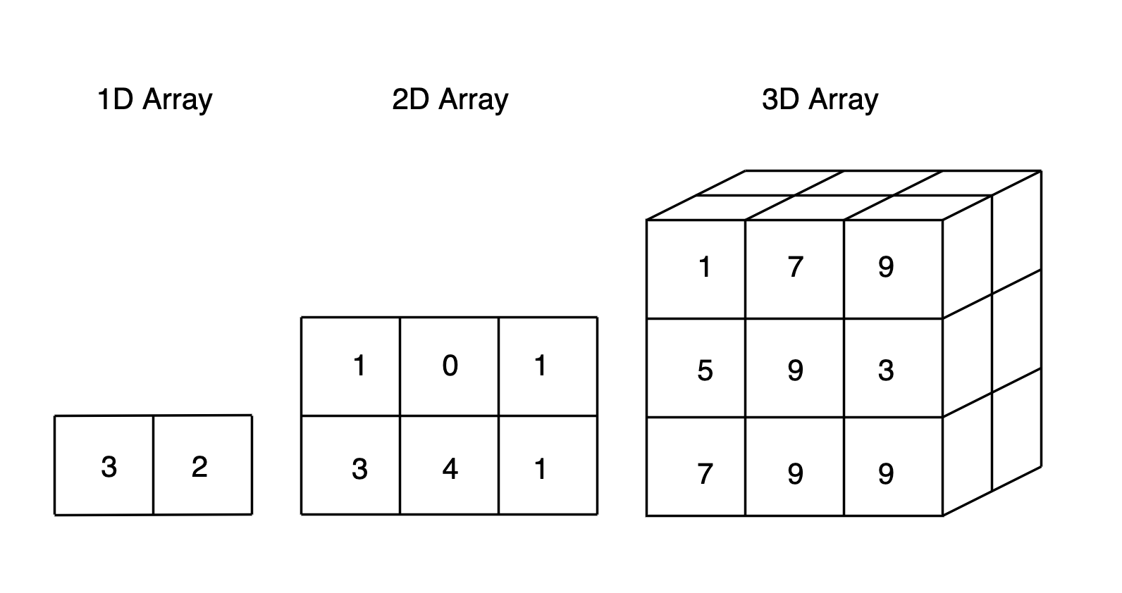
Arrays are one of the most conceptually straight-forward and common data structures. They may be one or multi-dimensional, and typically hold items of the same data type (such as integers, floats, strings, more arrays, etc.).

Arrays are indexed, which makes random access possible. They are, therefore, quite good for looking up values, and can also be useful for sorting. Arrays generally don’t take up much memory.

In some languages an array’s length is fixed and must be defined at the time of creation, which can be a problem. There can also be challenges with insertion and deletion, as we have to do lots of shifting of other elements.

Stacks

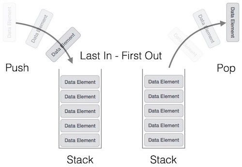
A stack is a LIFO (last in, first out) structure which resembles an array. An example would be an “undo” operation that stores previous states of work such that the most recent appears first. To get to a state in the middle, we’d need to undo all of the more recent states. One can think of the call stack for a concrete example.

Common operations include pushing a new element to the top of the stack, or popping and returning the topmost element off of a stack.

Queues

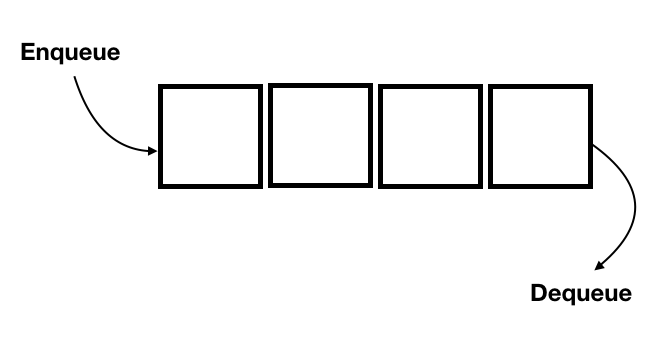
Queues are similar to stacks, except that they are a FIFO (first in, first out) structure. This is easy to conceptualize as a line of people waiting for something: The first person to arrive and stand in line is served first.

Common queue operations include enqueue, which inserts an element at the end of a queue, and dequeue, which deletes an element from the beginning of the queue.

Linked Lists

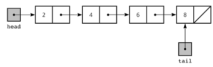
A linked list is a sequential structure that consists of items in linear order, which are linked to each other.

Linked lists differ from arrays in how they are stored in memory. As a simplification, with a fixed-length array, if we want to add an element and there is not sufficient memory right at the end of where it is stored, we have to copy the entire array to a new area with sufficient memory and delete the old one. With linked lists this is not necessary. However, random access is not possible with this data structure as there is no index.

Elements in a linked list are known as nodes. Each node is composed of a key, the actual value, and next, which is a pointer to the next node. The head is the first element of a linked list, and the tail is the last element (which has a next value of NULL).

There are several types of linked lists:

• Singly-linked lists: Elements can only be traversed moving forward.
• Doubly-linked lists: Elements can be traversed both forwards and backwards. Each node has an extra pointer known as prev which points to the previous node.
• Circular linked lists: The prev pointer of the head points to the tail, and the next pointer of the tail points to the head.

Trees

Like linked lists, trees are also composed of nodes. However, the nodes are organized hierarchically instead of linearly, and they are a-cyclical.

The top element is known as the root, and a terminating element is a leaf. Relationships between nodes are specified as parent/child/sibling. Parent and child nodes are quite obvious, and sibling simply refers to nodes with the same parent node.

A common tree example is a binary search tree, which is composed of nodes with up to two next pointers: left and right. Elements are sorted, with everything to the left being smaller, and to the right being larger. This allows for quite efficient searching at O(log n) time.

Heaps

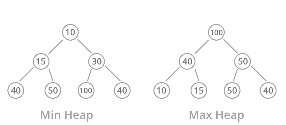
Heaps are a special type of binary tree-based data structure. They typically come in two types:

• Max heap: The value at each child node must be less than or equal to the value of the parent node, all the way through all subtrees. The greatest value is at the root.
• Min heap: The value at each child node must be greater than or equal to the value of the parent node, all the way through all subtrees. The smallest value is at the root.

Heaps are used when the highest or lowest order/priority element needs to be removed. They allow quick access to this item in O(1) time, but they only provide easy access to the smallest/greatest item. Finding other items in the heap takes O(n) time because the heap is not ordered, so we have to go through all the nodes.

Tries

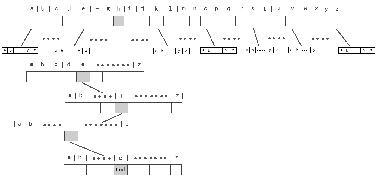
Tries are related to trees, but the name is actually short for “retrieval.” Basically, a trie is a tree whose nodes are arrays. Some nodes are shared between individuals, but each complete key will be unique.

Tries are memory intensive, but have O(1) constant time for search and insertion. For example, say we are interested in searching for a name in a trie of names: We would only need to search through each letter of the name, so the number of steps has a fixed upper bound based on the number of letters, and is therefore a constant.

Hash Tables

In a hash table, data are stored in an array format. What differentiates them is the use of “hashing,” whereby keys are transformed into array indices (“hash codes”) using a hash function. Each key then has associated values, like a dictionary. The key/value pairs are distributed uniformly across an array, and can be accessed using the key in O(1) time.

A hash function could pursue many different strategies to transform a key to a hash code. For example, if we were storing names we could take the modulo of the sum of the ASCII codes and the size of the array. If we had advanced knowledge of all possible keys it is theoretically possible to create a “perfect” hash function that uniquely assigns all keys without any ending up in the same place, but typically we will need to be more flexible.

In the case of collisions - where two or more keys end up in the same index position - we have some options:

• Open addressing: In this case, elements can be put somewhere other than their calculated address. For example, we could use linear probing and simply assign the element to the next free location in the array.
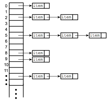
• Closed addressing: Alternatively, we can prohibit elements from being stored somewhere other than their calculated address. In such cases we can utilize chaining, where each array index is the head of a linked list.

With a closed addressing strategy, hash tables are simply arrays where each index leads to a linked list. This approach combines the advantage of random access with the ability for a data structure to grow and shrink.

Deleting and inserting data is easy with hash tables, and lookup is - on average - better than with linked lists. However, hash tables aren’t ideal if sorting is the goal, as one might as well just use an array in that case. They can also really run the gamut in terms of memory requirements.