Distance Measures for ML

What I Learned: Some Common Distance Measures, and When to Use Them.

Distance measures are used in machine learning for clustering and classification tasks. Generally speaking, a distance measure is an objective score that summarizes the relative difference between two objects, commonly rows of data that describe an observation.

There are MANY different distance measures (as evidenced by the 46 options in the R philentropy::distance() function), and choosing the most appropriate one is important, since they can have a strong influence on the results.

In some cases we may have different data types in one observational row, and different distance measures will have to be employed on each as appropriate and summed together to create a final score.

Another general note is that feature scaling is important for numerical distance measures.

Euclidean

Euclidean distance (also referred to as L2-Norm) is the most common distance measure, and is quite intuitive. It is simply the straight-line distance between two samples, and is the shortest possible distance between them.

It is used to calculate distance between numerical values, and is particularly sensitive to feature scale.

Mathematically, Euclidean distance is the square root of the sum of the squared differences between the two vectors.

Manhattan

Manhattan distance measures the point-to-point travel time, and is also referred to as City Block, Taxicab, or L1-Norm.

Manhattan distance is commonly used for binary predictors, and is advisable when dealing with high-dimensional data, or - if you are calculating errors - when you are interested in emphasizing outliers.

It is calculated as the sum of the absolute differences between the two vectors. For example, the Manhattan distance between [10, 20, 15] and [12, 18, 16] is 5.

Minkowski

Minkowski distance is a generalization of the Euclidean and Manhattan distances. Here, “generalization” means that we can manipulate the formula to calculate the distance between two data points in different ways.

Minkowski distance adds a parameter called the “order” or p, that allows different distance measures to be calculated. When p is set to 1, the calculation is the same as the Manhattan distance. When p is set to 2, it is the same as the Euclidean distance. In machine learning applications, p is a hyperparameter that can be tuned.

Mahalanobis

The Mahalanobis distance measure is useful when we have correlated variables, as it can take covariance into account. For example, in Euclidean space, the axes are orthogonal (drawn at right-angles), which implies a lack of correlation - therefore correlated variables cannot form a Euclidean space.

Mahalanobis distance measures the distance between a point and a distribution rather than between two distinct points. For uncorrelated variables this will equal Euclidean distance.

Hamming

Hamming distance is used for categorical variables, and measures whether the attributes of two observations are equal or not. It compares two equal-length arrays to determine where there are “mismatches” between elements at the same index.

For example, the Hamming distance between

[w, a, l, k]

[w, o, r, k]

is 2, because the 2nd and 3rd indices do not match. Similarly, the Hamming distance between

[1, 0, 1, 1, 0]

[1, 1, 1, 0, 1]

is 3, given the differences between the second, fourth, and fifth indices.

Cosine Similarity

Cosine similarity is a bit different in that we are now concerned with the vector angles rather than the magnitude. Mathematically, the cosine similarity measures the cosine of the angle between two vectors projected in a multi-dimensional space. Two vectors with the same orientation have a cosine similarity of 1. Two vectors at 90° have a similarity of 0. Two vectors diametrically opposed have a similarity of -1. This is regardless of their magnitudes.

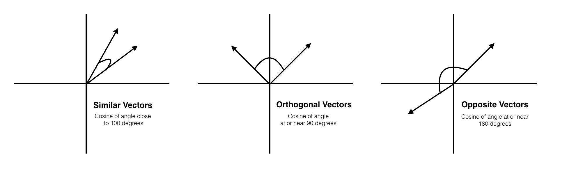
Cosine similarity is often used to compare documents and in recommendation systems.

Jaccard

Jaccard distance works with sets rather than vectors.

The cardinality of a set is just the number of elements contained in the set.

If we have two sets, A and B, the number of elements they have in common is the intersection \(A ∩ B\). The total set of elements in both sets is the union \(A ∪ B\).

Jaccard similarity is the cardinality of the intersection of two sets divided by the cardinality of the union of the sets.

\[|A ∩ B|/|A ∪ B|\]

For example, if set A is {cat, dog, hamster} and set B is {cat, pig, dog}:

\(A ∩ B\) = 2

\(A ∪ B\) = 4

The Jaccard similarity is 2/4 = 1/2