Mathematics for Machine Learning: Linear Algebra

Recently, I’ve been interested in going back to basics and working on getting a deeper understanding of the mathematical foundations behind machine learning and deep learning. To that end, I recently completed the Mathematics for Machine Learning: Linear Algebra course from Coursera, which I supplemented with some excellent linear algebra content from 3blue1brown.

The aim of this blog is to help me solidify my knowledge on the core topics from the course, and serve as a reference repository in case I happen to forget anything in the future. ;-) There were many more topics covered in more detail, of course, but these are the foundations that I want to make sure to remember moving forward.

So, why Linear Algebra? Most of the time in machine learning, data are represented in a matrix form. Understanding how mathematical operations are performed on matrices is therefore fundamental to understanding how machine learning models actually work. Some methods also draw directly on linear algebra (e.g. PCA, regularization, some recommendation systems), and understanding the math behind them is helpful for correct application, debugging, and even the development of new models.

Building Blocks

Scalars

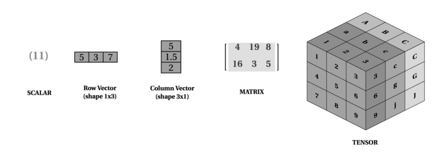
Scalars are simply a single number. The number 2 is a scalar, as is 13.455779, and so on.

Vectors

Vectors are “lists” or arrays of scalars. Each individual element in a vector is called a “component,” and represents a dimension in space.

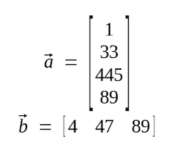
Vectors can be oriented either row or column-wise. In this example, both \(a\) and \(b\) are vectors (by convention, vectors are typically denoted with lowercase letters). \(a\) is a column vector with dimensions [4, 1], and \(b\) is a row vector with dimensions [1, 3].

The norm of a vector in vector space is a real non-negative value representing the length, size, or magnitude of the vector. There are different ways to measure this - two of the most common are:

• L2/Euclidean norm: This is the most commonly used norm, and is the cartesian distance between the vector elements.
• L1 norm: The sum of the absolute values of the vector’s elements.

Vector Operations:

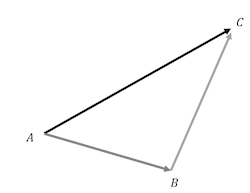
Addition: Numerically, we add two vectors by summing each of the individual elements. For example, \(a\) [1, 2, 3] + \(b\) [2, 3, 4] = \(c\) [3, 5, 7]. Geometrically, we can think of it as placing vector \(b\) to the end of \(a\), with the new vector \(c\) being the hypotenuse. Note that \(a + b\) is the same as \(b + a\).

Scalar Multiplication: Multiplying a vector by a scalar simply “scales” the vector by some degree, whether that be longer, shorter, or reverse. Numerically, one simply multiplies each component by the scalar. For example, 2 x [2, 4] = [4, 8].

As a geometric example, here the vector \(a\) is multiplied by the scalar 3:

Vector-Vector Multiplication (Dot Product): We can multiply two vectors in a couple of ways, though for me the simplest way is to multiply each component and add them together. The result is a scalar.

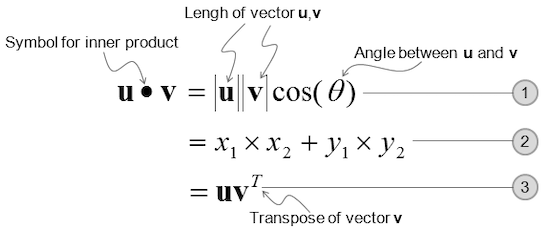
The dot product of two vectors tells us something about their angles:

• If the two vectors are orthogonal (at 90 degrees), the dot product will be zero.
• If they point in the same direction, the dot product will be positive.
• If they point in opposite directions, the dot product will be negative.

Matrices

A matrix is a two dimensional array of numbers. It can be thought of as two or more vectors stacked next to or on top of one another. Essentially, each column represents where one vector in a matrix “lands.”

If a matrix has m rows and n columns, then the order of the matrix is m x n. Elements in a matrix can be indexed using the row and column indices.

While matrices commonly represent a set of data points, they can also act as operators.

Types of Matrices

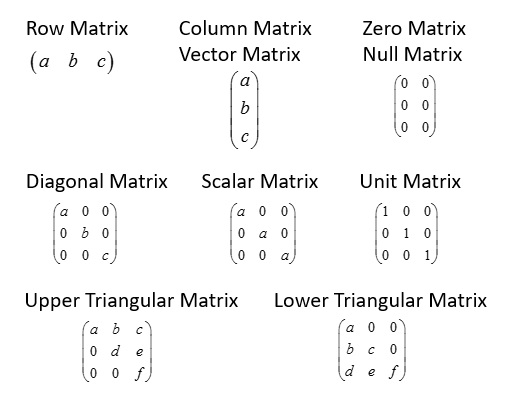
A few notable special matrices are:

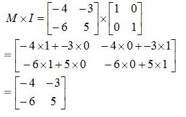
• Identity (or Unit) Matrix is a square matrix with ones on the diagonal, and zeroes everywhere else. It is unique in that multiplying a matrix by an identity matrix doesn’t change the original matrix.

• Scalar Matrix: Like an identity matrix, but with numbers other than one on the diagonal. In this case, the scalars on the diagonal are the amount that the vectors are scaled by, without changing the angles.

Matrix Operations

Examples in this section are largely taken from this useful blog.

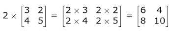
Matrix-Scalar Operations: To divide, multiply, add, or subtract a matrix by a scalar, simply do the operation on each element of the matrix. For example, multiplication:

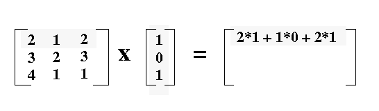
Matrix-Vector Multiplication: When multiplying a matrix by a vector, we’re essentially multiplying each row of the matrix by the vector column. The output is a vector with the same number of rows as the matrix.

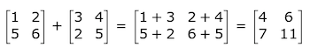
Matrix-Matrix Addition/Subtraction: To add matrices, they need to have the same dimensions. All that is required for matrix addition is to add each element at the same index together:

Matrix-Matrix Multiplication (Dot Product): This is only possible if the number of columns in the first matrix is the same as the number of rows in the second. This kind of matrix multiplication is referred to as the dot product, where every element of each row is multiplied by every element of each column, and added together.

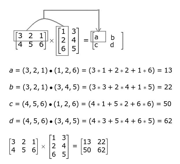
If the first matrix (\(A\)) is of shape(m, n), and is multiplied with matrix \(B\) of shape (n, p), the resulting matrix will be of shape(m, p).

There are some important properties of matrix multiplication:

• Not commutative: With scalars, 4 * 5 is the same as 5 * 4. This is not so with matrices, as AB does not equal BA. Multiplication by an identity matrix is an exception to this rule.
• Associative: Where the scalar multiplication 4(5 * 4) is the same as (4 * 5)4, with matrix multiplication \(A(B*C)\) is also the same as \((A*B)C\).
• Distributive: Like scalar multiplication, matrix multiplication is distributive. This means that 4(5 + 4) is the same as 4 * 5 + 4 * 4, and that \(A(B+C)\) is the same as \(A*B + A*C\).

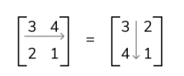
Matrix Transpose: Transposing a matrix is done by switching the rows and columns.

Matrix Inverse: An inverse of a scalar is whatever scalar you’d need to multiply that scalar by to equal the number one. Every number except zero has such an inverse. In the case of matrices, a matrix multiplied by its inverse results in an identity matrix.

Only square matrices can have inverses, and in some cases even square matrices don’t have any possible inverse (called singular or degenerate matrices). If the determinant (covered below) is zero, then the matrix isn’t invertible.

The matrix inverse is useful for solving systems of linear equations. We went through calculating inverse matrices and solving systems of linear equations using Gaussian Elimination by hand in the course, but in practice I’d likely just use numpy if it ever came up again.

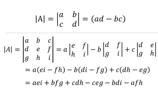
Determinants

The determinant of a square matrix is the factor by which it increases or decreases based on a linear transformation.

Whenever we invert the orientation of a matrix, the determinant will be negative. The absolute value still tells you the factor by which the area has been scaled, though. So a determinant of negative five means the space was scaled by a factor of five and inverted. It’s the same in three dimensions, except now we’re referring to how much volumes were scaled.

When the basis vectors (see below!) describing a matrix are not linearly independent, the determinant is zero. Basically, if the transformation squishes space into a smaller dimension (i.e. from a plane to a line), there is no transformation that can turn it back into a line. Same for 3D space onto a plane. This makes it impossible to solve systems of simultaneous equations or invert the matrix.

Tensors

Tensors weren’t covered in the course, but given their prevalence in deep learning applications, I thought it would be worthwhile to address them briefly as well.

Tensors are essentially generalizations of matrices, with potentially any number of dimensions. A 0D tensor is a scalar, a 1D tensor is a vector, and a 2D tensor is a matrix. Past 3D, we typically just refer to tensors.

There are also some other fancy properties of tensors related to transformations which distinguish them from general matrices. This is beyond the scope of this blog, but more info is available here.

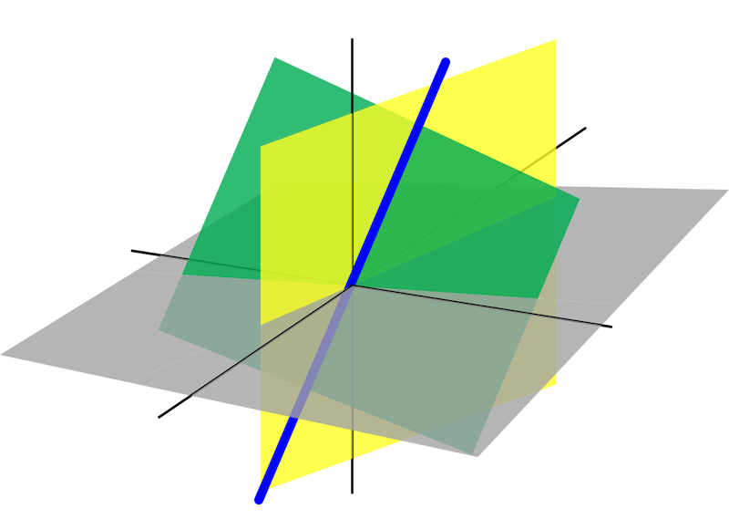
Span

The span of two vectors is the set of all possible vectors that you can reach with a linear combination of a given pair of vectors. It is basically a way of asking, “What are all the possible vectors you can reach using only two fundamental operations, vector addition and scalar multiplication?” For two linearly independent vectors, the span is a 2D plane (if they were linearly dependent, it would be a line).

The concept is the same for three+ vectors, except we obviously expand the space to three+ dimensions as well.

Note: If you can add an additional vector without changing the span, you can say these vectors are linearly dependent, as one of the vectors can be expressed as a linear combination of the others. If adding another vector adds another dimension, these vectors are linearly independent.

Basis Vectors

We use some coordinate system to define the direction of our vectors in space. These are the basis vectors.

Any time we describe vectors numerically, these values depend on what basis vectors we use, and are meaningful only if we know the basis vectors (though the vector exists without the basis independently as well).

The basis vectors must be linearly independent, and span the space. The number of basis vectors define the number of dimensions we’re working with.

Sometimes we may want to “translate” our basis into someone else’s, or vice versa. This video is an excellent overview of this topic.

A set of basis vectors that are all perpendicular to each other are called orthonormal. The matrix composed of them is called an orthogonal matrix. Ideally, we always want our transformation matrices to be orthogonal: This way the inverse is easy to compute, the transformation is reversible, and so on. The course presented the Gram-Scmidt process for constructing an orthonormal basis vector set.

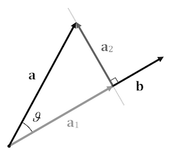
Projection

Imagine we have two vectors, \(a\) and \(b\). If we think of light shining down from perpendicular to \(b\), we get the projection of \(a\) onto \(b\). This gives us some information about the direction of the vectors (for example, if the vectors are orthogonal, the vector projection will be zero). The scalar projection is the length of the vector projection.

Projections are commonly used in linear algebra calculations. For data science in particular, we can think of a specific application of efficiently storing data, as described in this video. The algebra behind calculating vector projections is also derived clearly in the video.

Eigenthings

Eigenvectors are vectors that don’t get tilted off of their span when transformed. The eigenvalue is the factor by which an eigenvector is stretched or squished during the transformation. Conceptually, that’s basically it!

Some transformation matrices have no eigenvectors, and sometimes we may have multiple eigenvectors for one eigenvalue. For example, if we scaled all vectors by two, this uniform scaling means that all the vectors would be eigenvectors of this transformation. Rotations usually result in no eigenvectors, except for when rotating 180 degrees (giving eigenvalues of negative one).

I’m not going to cover calculating eigenvectors and values here, as this is unlikely to come up in the future. Conceptually, though, understanding Eigenthings is quite relevant for applications like PCA, or when we want to apply the same transformation matrix to different vectors multiple times.